Geometry and Linear Algebraic Operations
1. Geometry of vectors
- Vector is a list of numbers
- There are two types of vector: column vector, row vector
- data examples → column vectors
- Although column vector is default, for making tabular dataset we can treat data examples as row vector in the matrix conventionally
- weights used to form weighted sums → row vectors
- data examples → column vectors
- geometric interpretations of vectors
- points in space
- directions in space
points in space
- considering tasks as collections of points in space
- picturing the tasks as discovering how to seperate two distinct clusters of points
directions in space
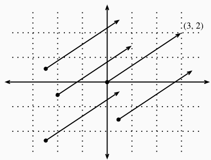
- v = [3, 2] → the location 3 units to the right and 2 units up from the origin (3 step to the right and 2 step up)

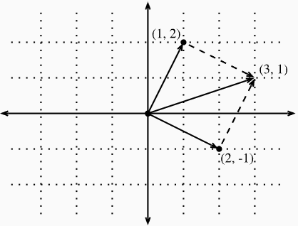
- visualizing vector addition by following the directions given by one vector, and then following the directions given by the other

2. Dot Products and Angles
Dot Product
- $\mathbf{u}^{\top} \mathbf{v}=\sum_{i} u_{i} \cdot v_{i}$
- $\mathbf{u} \cdot \mathbf{v}=\mathbf{u}^{\top} \mathbf{v}=\mathbf{v}^{\top} \mathbf{u}$ (the notation of classical multiplication)
geometric interpertation : dot product is closely related to the angle between two vectors

- consider two vectors v (length=r), w (length=s) → $\mathbf{v}=(r, 0)$ and $\mathbf{w}=(s \cos (\theta), s \sin (\theta))$
- $\mathbf{v} \cdot \mathbf{w}=r s \cos (\theta)=\|\mathbf{v}\|\|\mathbf{w}\| \cos (\theta)$
- $\theta=\arccos \left(\frac{\mathbf{v} \cdot \mathbf{w}}{\|\mathbf{v}\|\|\mathbf{w}\|}\right)$
import torch

def angle(v, w):
  return torch.acos(v.dot(w) / (torch.norm(v) * torch.norm(w)))

angle(torch.tensor([0, 1, 2], dtype=torch.float32), torch.tensor([2.0, 3, 4])) #tensor(0.4190)
※ orthogonal
$\theta=\pi / 2$ ($\theta=\pi / 2$) is same thing as $\cos (\theta)=0$
two vectors are orthogonal if and only if $\mathbf{v} \cdot \mathbf{w}=0$
"why is computing the angle useful?"
Consider an image and a duplicate image, where every pixel value is the same but 10% the brightness
- If we calculate the distance between the original image and the darker one, the distance can be large
- If we consider the angle, for any vector v, the angle between v and 0.1⋅v will be zero
- Scaling vectors keeps the same direction and just changes the length
2.1. Cosine Similarity
Cosine Similarity is used when the angle is employed to measure the closeness of two vectors,
$$
\cos (\theta)=\frac{\mathbf{v} \cdot \mathbf{w}}{\|\mathbf{v}\|\|\mathbf{w}\|}
$$
- two vectors poin in the same direction → maximum value of 1
- two vectors point in opposite directions → minimum value of 1
- two vectors are orthogonal → a value of 0
- if the components of high-dimensional vectors are sampled randomly with mean 0, their cosine will nearly always be close to 0
3. Hyperplanes
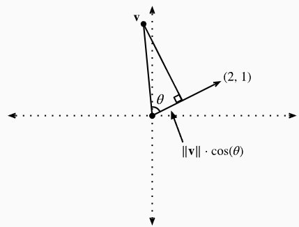
“what are the points v with w⋅v=1 ?”
$$
\|\mathbf{v}\|\|\mathbf{w}\| \cos (\theta)=1 \Longleftrightarrow\|\mathbf{v}\| \cos (\theta)=\frac{1}{\|\mathbf{w}\|}=\frac{1}{\sqrt{5}}
$$

- $\|\mathbf{v}\| \cos (\theta)$ is the length of the projection of the vector v onto direction of w
- y = 1 - 2x


Based on the orthogonal point v · w = 1, when it is v · w > 1, it is more similar to a vector(2, 1) and when it is v · w < 1, it is less similar to a vector (2, 1)
4. Geometry of Linear Transformations
a geometric understanding of linear transformations represented by matrices is also important
$$
\mathbf{A}=\left[\begin{array}{ll}
a & b \\
c & d
\end{array}\right]
$$
we multiple $\mathbf{v}=[x, y]^{\top}$
$$
\begin{aligned}
\mathbf{A} \mathbf{v} &=\left[\begin{array}{ll}
a & b \\
c & d
\end{array}\right]\left[\begin{array}{l}
x \\
y
\end{array}\right] \\
&=\left[\begin{array}{l}
a x+b y \\
c x+d y
\end{array}\right] \\
&=x\left[\begin{array}{l}
a \\
c
\end{array}\right]+y\left[\begin{array}{l}
b \\
d
\end{array}\right] \\
&=x\left\{\mathbf{A}\left[\begin{array}{l}
1 \\
0
\end{array}\right]\right\}+y\left\{\mathbf{A}\left[\begin{array}{l}
0 \\
1
\end{array}\right]\right\}
\end{aligned}
$$
For example,
$$
\mathbf{A}=\left[\begin{array}{cc}
1 & 2 \\
-1 & 3
\end{array}\right]
$$
$$
\mathbf{v}=[2,-1]^{\top}
$$
- $\mathbf{v}=2 \cdot[1,0]^{\top}+-1 \cdot[0,1]^{\top}$
- the matrix A will send vector v to $2\left(\mathbf{A}[1,0]^{\top}\right)+-1(\mathbf{A}[0,1])^{\top}=2[1,-1]^{\top}-[2,3]^{\top}=[0,-5]^{\top}$

- All matrices can do is take the original coordinates on our space and skew, rotate, and scale them
5. Linear Dependence
consider specific matrix B
$$
\mathbf{B}=\left[\begin{array}{ll}
2 & -1 \\
4 & -2
\end{array}\right]
$$
This compresses the entire plane down to live on the single line y = 2x
- $\mathbf{b}_{1}=[2,4]^{\top}$
- $\mathbf{b}_{2}=[-1,-2]^{\top}$
- transformed by the matrix BB as a weighted sum of the columns of the matrix $a_{1} \mathbf{b}_{1}+a_{2} \mathbf{b}_{2}$ → linear combination
- $\mathbf{b}_{1}=-2 \cdot \mathbf{b}_{2}$
$$
a_{1} \mathbf{b}_{1}+a_{2} \mathbf{b}_{2}=-2 a_{1} \mathbf{b}_{2}+a_{2} \mathbf{b}_{2}=\left(a_{2}-2 a_{1}\right) \mathbf{b}_{2}
$$
$$
\mathbf{b}_{1}+2 \cdot \mathbf{b}_{2}=0
$$
a collection of vectors $\mathbf{v}_{1}, \ldots, \mathbf{v}_{k}$ are linearly dependent if there exist coefficients $a_{1}, \ldots, a_{k}$ not all equal to zero
$$
\sum_{i=1}^{k} a_{i} \mathbf{v}_{\mathbf{i}}=0
$$
- a linear dependence in the columns of a matrix is a witness to the fact that our matrix is compressing the space down to some lower dimension
- If there is no linear dependence we say the vectors are linearly independent ($a_{1}, \ldots, a_{k}$ all equal to zero). If the columns of a matrix are linearly independent, no compression occurs and the operation can be undone
6. Rank
- Rank: maximum number of linearly independent vectors
- Column Rank: maximum number of linearly independent column vectors.
- Row Rank: maximum number of linearly independent row vectors.
$$
\mathbf{B}=\left[\begin{array}{ll}
2 & 4 \\
-1 & -2
\end{array}\right]
$$
▶ rank(B)=1
7. Invertibility
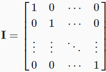
multiplication by a full-rank matrix (i.e., someA that is n×n matrix with rank n), we should always be able to undo it

When the above equation is satisfied, A is called invertable matrix and A-1 is called the inverse matrix

Consider specific matrix A

The inverse matrix is calculated as follows

8. Determinant

- determinant = ad−bc
- a matrix A is invertible if and only if the determinant is not equal to zero
import torch

torch.det(torch.tensor([[1, -1], [2, 3]], dtype=torch.float32)) #tensor(5.)
[reference]